Overview

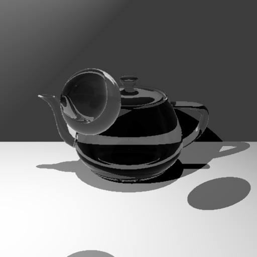
As part of the Advanced Computer Graphics module (CM30075), I built a ray tracer from scratch in C++ capable of rendering complex scenes with physically-based lighting. The renderer supports multiple primitive types; spheres, planes, quadratic surfaces, and .obj polymesh files. it also implements a range of advanced rendering techniques including reflection, refraction, texture mapping, anti-aliasing, and photon mapping.

---

Reflection and Refraction

To render transparent and reflective surfaces, the renderer computes both a reflected and a refracted ray at each intersection point, then blends them using the Fresnel equations.

Reflection follows the law of reflection, the angle of incidence equals the angle of reflection:

r' = r - 2(r · n)n

Refraction is computed via Snell's Law, using a per-material index of refraction (IOR) to control how much the ray bends. A value of 1.0 represents air, 1.5 represents glass. A special case total internal reflection is handled by detecting when the discriminant goes negative, at which point the ray reflects instead of refracting.

The Fresnel equations determine the ratio of reflected ($K_r$) to transmitted ($K_t$) light, and the final pixel colour is blended accordingly:

final colour = Kr × reflected colour + Kt × refracted colour

Both reflected and refracted rays are traced recursively, with a maximum depth limit to prevent infinite bounces and discard rays that contribute negligibly to the final image.

---

Quadratic Surfaces

The renderer supports any quadratic implicit surface defined by the general form:

Ax² + 2Bxy + 2Cxz + 2Dx + Ey² + 2Fyz + 2Gy + Hz² + 2Iz + J = 0

This covers spheres, cylinders, cones, paraboloids, and hyperboloids. Ray–surface intersection is solved by substituting the parametric ray equation into the quadratic, yielding a standard discriminant test. Surface normals are computed analytically at the intersection point.

Transformations (translation, rotation, scale) are applied by transforming the quadratic matrix directly:

Q' = TᵀQT

This avoids having to transform every ray and keeps the intersection logic general.

---

Texturing

Texture mapping is implemented via a TextureMaterial class that loads JPEG images using the stb_image.h library and stores them as a pixel array. At intersection time, the material retrieves the $(s, t)$ UV coordinates from the hit record and maps them to pixel coordinates for colour lookup.

UV coordinates are computed differently per object type:

• Sphere: Derived from spherical coordinates $(\theta, \phi)$ at the intersection point, normalised to $[0, 1]$.
• Polymesh: UV values are read directly from the .obj file per vertex, then interpolated across triangles using barycentric coordinates at the intersection point.
• Plane: A partial implementation using world-space $(x, y)$ position, not fully satisfactory due to the unbounded nature of planes.

---

Anti-Aliasing

Aliasing is reduced using an adaptive supersampling strategy. Rather than applying multi-sample rendering uniformly across every pixel (which is expensive), the renderer does it in two passes:

1. Edge detection pass: An initial single-sample render is produced. For each pixel, the Euclidean colour distance to its neighbours is computed and averaged. This identifies pixels that sit on or near a geometric edge.

2. Supersampling pass: Pixels whose average neighbour distance exceeds a threshold of 0.5 are re-rendered with 4 additional jittered samples (top-left, top-right, bottom-left, bottom-right offsets of ±0.5). The 5 samples are averaged to produce the final colour.

This focuses rendering cost where it matters, significantly improving edge quality while keeping render times practical.

---

Photon Mapping

Photon mapping is a two-pass global illumination algorithm that simulates how light energy propagates and accumulates throughout a scene.

Pass 1 — Photon Tracing

Photons are emitted from point light sources in uniformly random directions. Each photon carries a colour intensity and is traced through the scene. At each intersection, the material uses Russian Roulette to probabilistically decide whether the photon is absorbed, reflected, or refracted — with intensities scaled by the inverse probability to keep the estimator unbiased.

Two separate photon maps are maintained:

• Diffuse map: Photons that have hit a diffuse surface.
• Caustic map: Photons that have undergone at least one specular interaction (reflection or refraction through a transparent object) before hitting a diffuse surface. To increase caustic density, additional photons are seeded randomly within the radius of each caustic hit point and re-traced.
• Shadow photons: Traced from each first-bounce intersection toward the light source to improve shadow accuracy.

All photons are stored in a KD-Tree (nanoflann library) for efficient nearest-neighbour lookup. Recent query results are cached to avoid redundant searches for nearby points.

Pass 2 — Radiance Estimation

During the main ray trace, when a ray hits a diffuse surface, the $k$ nearest photons are gathered from the KD-Tree. Radiance is estimated using Gaussian kernel density estimation (following Jensen's SIGGRAPH 2000 practical guide), weighting each photon by its distance:

wᵢ = α [ 1 - (1 - exp(-β · dp² / 2r²)) / (1 - exp(-β)) ]

with α = 0.918 and β = 1.953. The weighted photon contributions are added to the direct illumination already computed by the ray tracer.

Note: The photon mapping implementation is partial — direct illumination and photon tracing work correctly, but the caustic radiance estimation did not produce the expected focused caustic patterns despite experimenting with varying $k$-nearest-neighbour counts, photon counts, and search radii.

---

Key Outcomes

• Full ray tracer implemented in C++ from scratch, no external rendering libraries
• Supports spheres, planes, .obj polymesh files, and arbitrary quadratic surfaces
• Physically-based reflection and refraction with Fresnel blending and recursive depth control
• UV texture mapping across multiple primitive types with barycentric interpolation for meshes
• Adaptive anti-aliasing focusing supersampling cost on geometric edges
• Two-pass photon mapping with separate caustic and diffuse maps, KD-Tree storage, and Gaussian radiance estimation

---

Reflections

Building a renderer from first principles forces a close engagement with the mathematics of light transport that higher-level tools abstract away. Deriving and implementing Snell's Law, the Fresnel equations, and the quadratic intersection formula by hand makes the tradeoffs in physically based rendering concrete.

The photon mapping implementation was the most challenging part. Getting the first pass (emission and storage) working was straightforward; the radiance estimation in the second pass is sensitive to the interplay between photon count, search radius, and kernel bandwidth in ways that are difficult to debug visually. With more time I would instrument the photon map density directly.

Adaptive anti-aliasing was a satisfying optimisation: the edge-detection heuristic is simple but effective, and the visual improvement over no anti-aliasing is immediately apparent at object silhouettes and shadow boundaries.